Adaptive Random Testing Introduction

A step-by-step guide.

Nov 13, 2025

This is a practical explanation of adaptive random testing (ART). We’ll build intuition with tiny, concrete examples. At the end of this post, I will give a brief example using Python.

Code: https://github.com/khaled-e-a/semantics-systems/tree/main/art-1

Concept overview

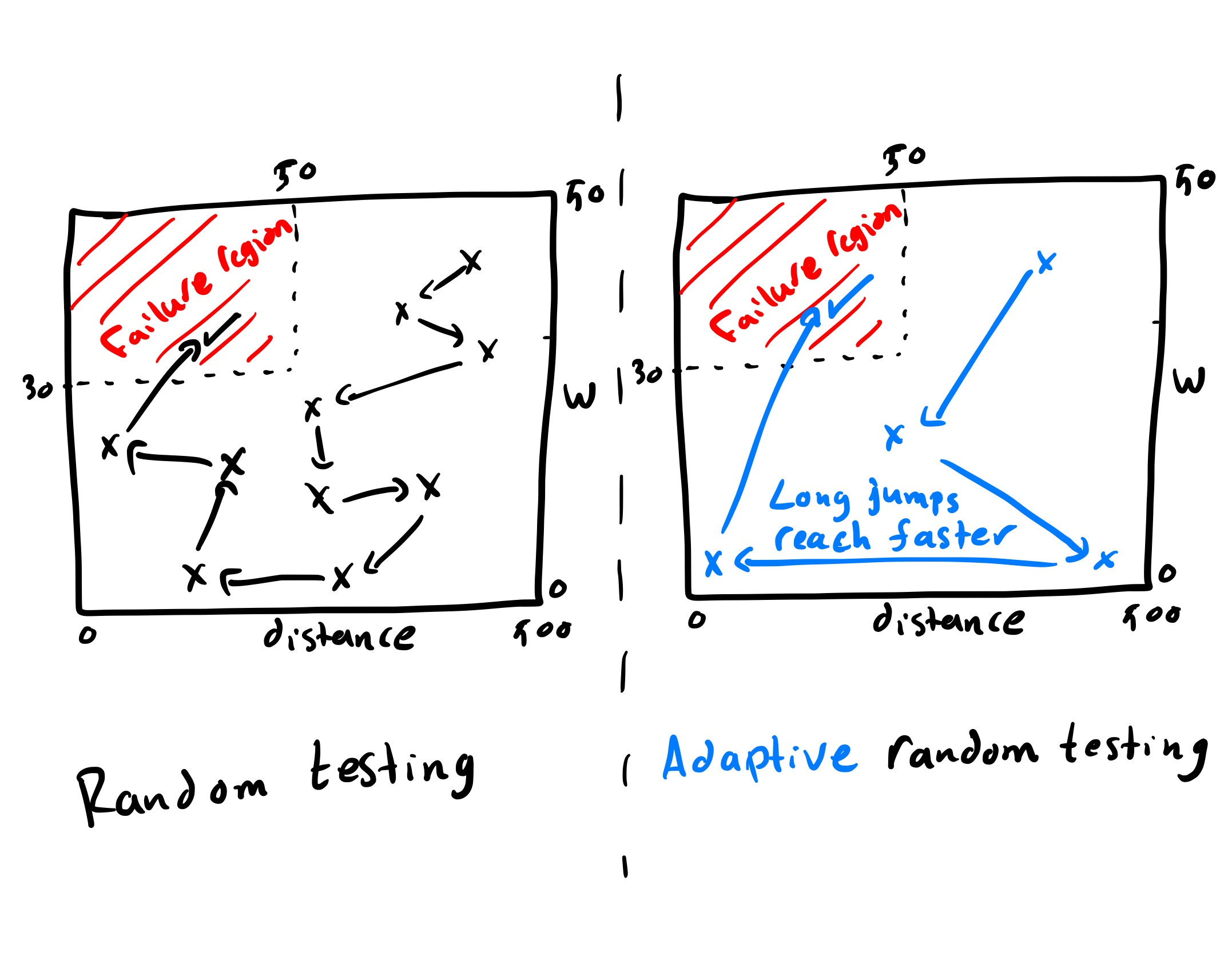
Random testing selects inputs uniformly at random from the input domain and executes the program under test. This approach is attractive because it is simple to implement and easy to scale, but it suffers from a structural problem: test inputs tend to cluster in some parts of the domain while leaving other parts untested.

Adaptive Random Testing (ART) preserves the use of random generation while explicitly trying to avoid such clusters. The core principle is to keep test cases well spread across the input space, to avoid large “holes” in coverage.

This principle is motivated by a common empirical observation about software faults:

Failure-causing inputs often form contiguous regions in the input domain rather than isolated points.

If failures cluster in regions, then a test set that covers the domain more evenly yields a higher probability that at least one test will fall inside a failure region early.

The Fixed-Size Candidate Set (FSCS) algorithm is the classical and simplest instance of ART. FSCS translates the informal idea “select the next test far from previous ones” into a concrete distance-based selection rule.

Motivating example

Consider an online shipping service that takes two numeric inputs:

weight_kg in the range from 0 to 50
distance_km in the range from 0 to 500

The service computes a shipping price as a base fee plus terms that scale with weight and distance. Marketing requests a discount policy: when the package is heavy (weight greater than 30 kg) and the delivery is long distance (distance greater than 300 km), the service should apply a 10 percent discount.

Assume a bug is introduced during implementation. Instead of checking distance_km > 300 for the discount rule, the code checks distance_km < 50 and applies a very large discount that can make the final price negative.

This bug creates a rectangular failure region in the two-dimensional input space.
Any input with weight_kg > 30 and distance_km < 50 lies inside this region and produces a negative price, which is clearly incorrect.

If we use plain random testing, we repeatedly sample (weight_kg, distance_km) uniformly from the domain.
By chance, many tests may focus on light or medium weights or on medium and long distances, so the region of heavy and very short-distance shipments may remain untested for a long time.

In contrast, an ART strategy that prefers inputs far from those already used will progressively push tests into previously unexplored parts of the weight–distance plane.
This spreading effect makes it much more likely that a test will eventually enter the “heavy and short distance” rectangle and expose the negative-price failure.

ART Approach

The central objective of ART is to obtain an even spread of tests over the input domain.
Informally, if we plot all test points, they should occupy the space in a balanced way, with few dense clusters and few large empty regions.

FSCS-ART formalizes this idea using distances between test inputs.
Each input is treated as a point in a multidimensional space, and a distance function measures how close or far two points are; in the shipping example, each test is a point (weight_kg, distance_km), and Euclidean distance on appropriately normalised coordinates is a natural choice.

FSCS maintains:

a set E of executed tests, and
a fixed-size set C of randomly generated candidates for the next test.

The algorithm proceeds as follows.

First, the initial test input is chosen uniformly at random from the input domain and added to E.
At this point, there is no information about the space, so simple random selection is sufficient.

For each subsequent test, FSCS generates a small number of random candidates and places them into C.
For each candidate c in C, the algorithm computes the distance from c to its nearest neighbour in E.

FSCS chooses as the next test the candidate whose nearest-neighbour distance is largest among all candidates, which means it selects the candidate that lies in the “emptiest” neighbourhood relative to the tests run so far.

This rule has a simple geometric effect on the test set. Each new test is placed into a region that is far from existing tests, so over time, the distribution of tests becomes more uniform and holes in coverage are progressively filled.

In the shipping example, if early tests concentrate on light packages and medium or long distances, then candidates near those areas will have small nearest-neighbour distances.
FSCS will tend to reject such candidates in favour of those in sparsely tested regions, and eventually selects a candidate in the heavy short-distance rectangle that reveals the bug.

Example code & output

First, clone the code examples repo. The example is in the art-1 directory. You can then run the example from the command line as follows:

python fscs_art_demo.py --tests 40 --candidates 10 --seed 0

The --tests option sets the maximum number of test cases, --candidates sets the size of the FSCS candidate set, and --seed sets the random seed for reproducibility.

The code has three main roles: it defines the 2D input domain and distance functions, implements the shipping-cost system with the injected bug, and implements FSCS-ART plus a small test harness that prints each test and stops once a failure is found.

Each test case is printed on a single line in this format:

idx: weight=WW.WW kg, distance=DDD.D km, nearest_distance=R.RRR, result=PASS/FAIL

The weight and distance fields show the concrete input, nearest_distance is the distance to the closest previous test in the normalised space, and result reports whether this input exposed a failure (negative price) or not.

At the end, the script prints a short summary indicating whether a failure was found and, if so, after how many tests.
When FSCS is effective, the failing input usually has a heavy weight and a short distance, which confirms that the algorithm has driven the search into the buggy “heavy and short-distance” region of the domain.

Practical considerations

Distance metric. For numeric inputs, Euclidean distance on normalised dimensions is often adequate, but for other domains, one may choose Hamming distance, edit distance, or a problem-specific structural or behavioural distance.
Candidate set. A larger candidate set improves the chance that one candidate falls in a genuinely unexplored region, although it also increases the number of distance computations at each step; in practice, modest sizes such as 5 to 20 candidates usually provide a good balance between diversity and overhead.
Computational cost. At step i, FSCS compares each candidate in C to all i − 1 previously executed tests in E, so naïve implementations incur a cost that grows with both the number of tests and the candidate set size.
Several engineering tactics can reduce this cost without changing the core idea of diversity. Examples include abandoning very old tests that are no longer relevant to local spacing, or using approximate distance computations when exact distances are unnecessary.

Finally, the effectiveness of ART depends on how failures are distributed in the input space. When failure regions are contiguous, even spreading tends to reduce the expected number of tests required to find at least one failing input, while for isolated point-like failures, the benefit is smaller and may not justify the extra overhead.

Conclusions

Adaptive Random Testing enhances random testing by incorporating a very small amount of structure: it remembers past tests and steers new tests away from already explored regions. The FSCS algorithm offers a clear and compact realization of this idea through its “farthest candidate” selection rule.

In the shipping-cost example, this rule directs testing toward regions of the weight–distance space that have not yet been exercised and consequently leads to earlier discovery of the failure region associated with the discount bug. This behaviour illustrates the general advantage of diversity-oriented test generation when failures are expected to cluster.

For practitioners, the takeaway is that improving the spatial diversity of tests can significantly increase the chance of exposing faults without abandoning the simplicity of random generation. FSCS-ART provides a practical and easy-to-explain starting point for adding this kind of diversity to existing testing workflows.

Semantics & Systems

Discussion about this post